Import Libraries

Import the necessary libraries for data analysis and visualisation.

    ```{r message=FALSE, warning=FALSE, error=TRUE}
    # load packages
    library(ggplot2)
    library(readr)
    library(dplyr)
    ```
                

Data Inspection

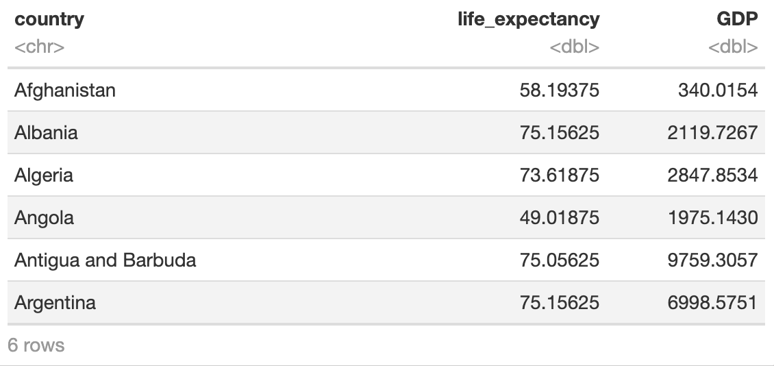
Look at the head of the dataset to have an idea of the information the dataset give you.

    ```{r error=TRUE}
    # import and inspect data
    data <- read_csv("country_data.csv")
    head(data)
    ```
                

Life Expectancy Analysis

Find the quartiles of the data in order to get an idea of how the data is spread.

    ```{r error=TRUE}
    # life expectancy
    life_expectancy <- data %>% pull(life_expectancy)
    # life expectancy quartiles
    life_expectancy_quartiles <- quantile(life_expectancy, c(0.25, 0.5, 0.75))
    print(life_expectancy_quartiles)
    ```
                

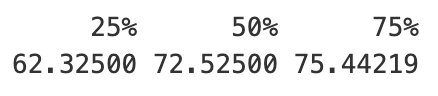
From the quartiles, we can see that the median life expectancy is 72.52 years, with the first quartile being 62.33 years and the third quartile being 75.44 years.

This means that 50% of countries have a life expectancy between 62.33 and 75.44 years.

Next, I will create a histogram to visualise the distribution of life expectancy across countries.

    ```{r error=TRUE}
    # plot histogram of life expectancy
    hist(life_expectancy)
    ```
                

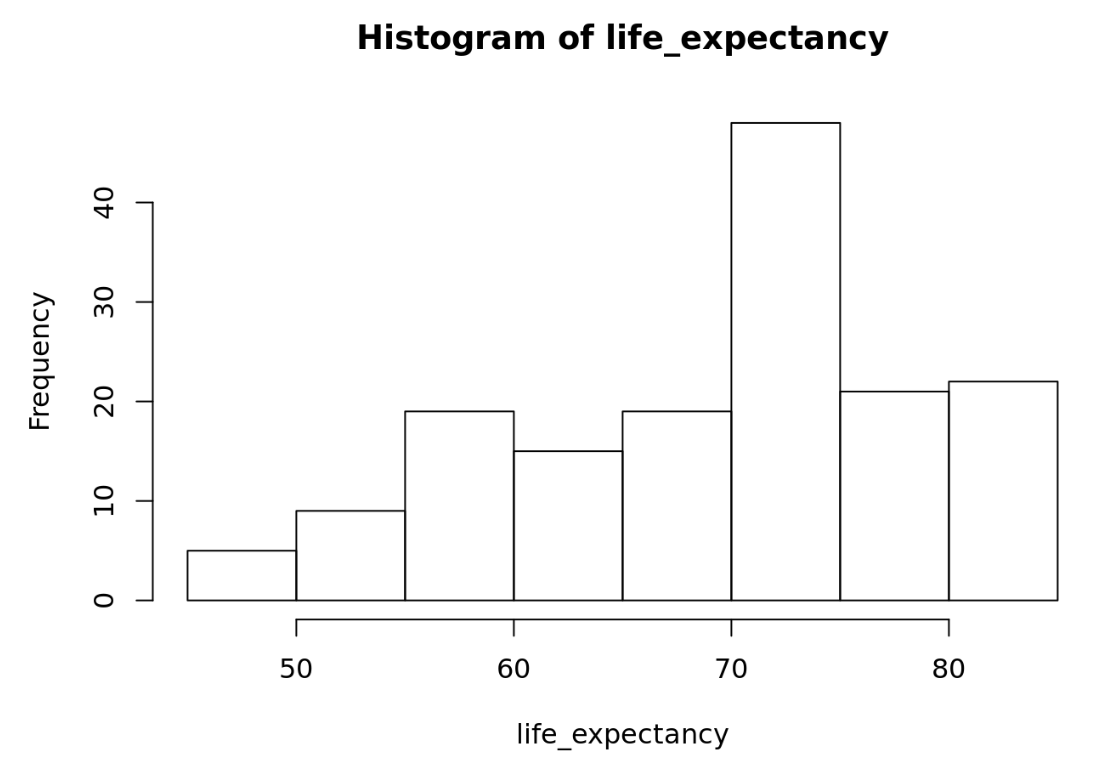
The histogram shows that the life expectancy is right-skewed, with a majority of countries having a life expectancy between 60 and 80 years.

GDP Data Analysis

Next, I will look at the GDP data to see how it is distributed.

First I shall split the data into two groups, the low GDP which are the countries that are less than or equal to the median and the high GDP which are the countries greater than the median.

In order to do this I must first find the median.

    ```{r error=TRUE}
    # gdp
    gdp <- data %>% pull(GDP)
    head(gdp)
    # median gdp
    median_gdp <- median(gdp)
    print(median_gdp)
    ```
                

The median GDP is 2938.078.

Now I can split the data into two groups, the low GDP and high GDP.

I shall first look at the low GDP and find the quartiles of that data.

    ```{r error=TRUE}
    # low gdp
    low_gdp <- data %>% filter(GDP <= median_gdp) %>% pull(life_expectancy)
    # low gdp quartiles
    low_gdp_quartiles <- quantile(low_gdp, c(0.25, 0.5, 0.75))
    print(low_gdp_quartiles)
    ```
                

Now I shall look at the high GDP and find the quartiles of that data.

    ```{r error=TRUE}
    # high gdp
    high_gdp <- data %>% filter(GDP > median_gdp) %>% pull(life_expectancy)
    # high gdp quartiles
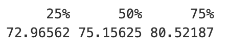
    high_gdp_quartiles <- quantile(high_gdp, c(0.25, 0.5, 0.75))
    print(high_gdp_quartiles)

    ```
                

From the quartiles, we can see that the median life expectancy for low GDP countries is 64.34 years, with the first quartile being 56.34 years and the third quartile being 71.74 years.

For high GDP countries, the median life expectancy is 75.16 years, with the first quartile being 72.97 years and the third quartile being 80.52 years.

This means that 50% of low GDP countries have a life expectancy between 56.34 and 71.74 years, while 50% of high GDP countries have a life expectancy between 72.97 and 80.52 years.

Next, I will create histograms to visualise the distribution of life expectancy for both low and high GDP countries.

    # plot low gdp histogram
    hist(low_gdp, xlab="Life Expectancy", col='red')
    # plot high gdp histogram
    hist(high_gdp, xlab="Life Expectancy", col='blue')
    ```
                

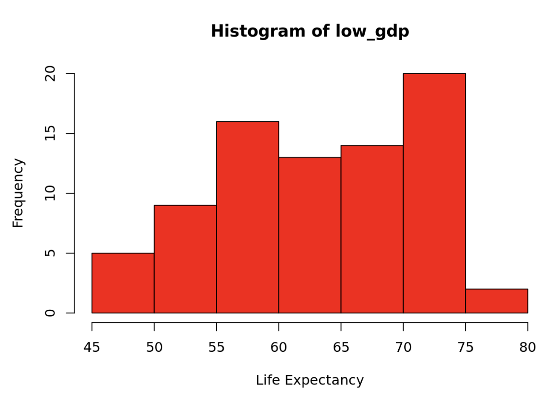
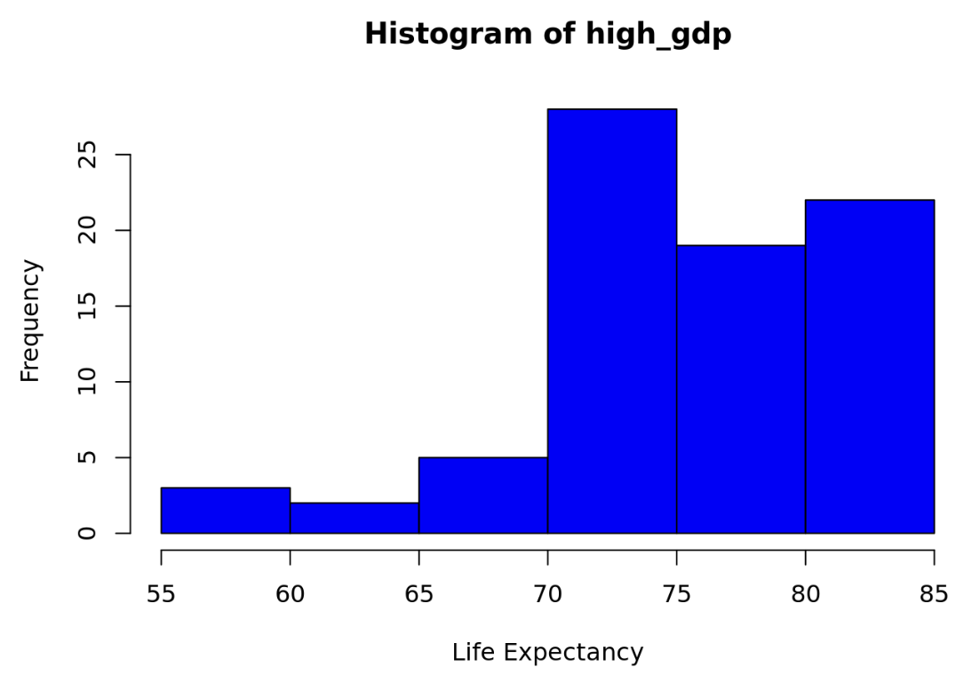
The histograms show that the life expectancy for low GDP countries is slightly left-skewed skewed, however the life expectancy for high GDP countries is very left-skewed, with a majority of countries having a life expectancy between 70 and 85 years.