Traffic Safety Data Analysis Project

This project involves analysing traffic safety data and smartphone usage to identify patterns and trends.

The goal is to use Python to process and visualise the data, providing insights on if there is a correlation between smartphone usage and traffic accidents.

The first dataset can be found on the National Highway Traffic Safety Administration’s website.

The second dataset can be found on the Pew Research Center’s website.

Project Hypothesis

My hypothesis is that as smartphone usage increases, the number of traffic accidents will also increase due to distracted driving.

Project Method

Import Libraries

Import the necessary libraries for data analysis and visualisation.


    import pandas as pd
    import datetime as dt
    from scipy.stats import pearsonr
    from sklearn.linear_model import LinearRegression
    import seaborn as sns
    import matplotlib.pyplot as plt


    %matplotlib inline
    # set plot theme and palette
    sns.set_theme()
    sns.set_palette('colorblind')

Traffic Safety Data Inspection

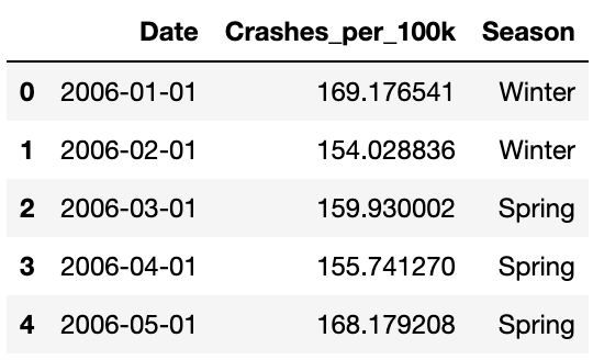
Look at the head of the dataset to have an idea of the information the dataset give you.


    traffic=pd.read_csv('traffic.csv')
    traffic.head()

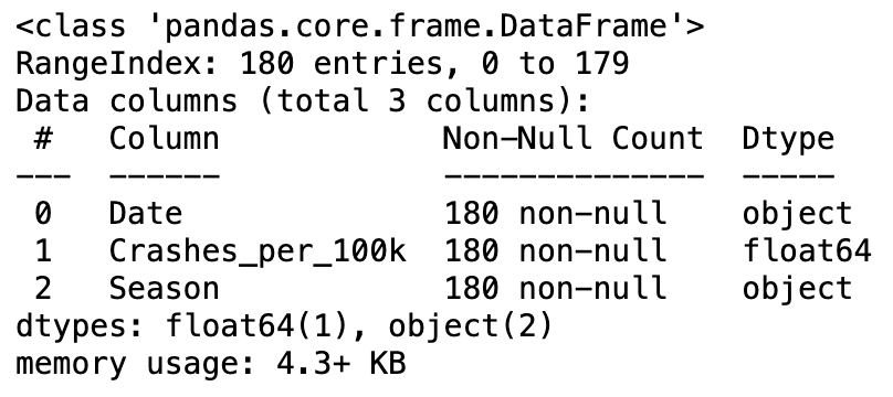
Check the datatypes of the columns to ensure they are correctly formatted.


    traffic.info()

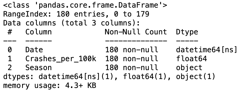
Change the datatype of the 'Date' column to datetime format.


    traffic['Date']=pd.to_datetime(traffic['Date'])
    traffic.info()

Traffic Safety Analysis

Hypothesis

My hypothesis is that the number of crashes will increase over the years as I believe cars are more affordable and therefore more cars are on the road.

Method

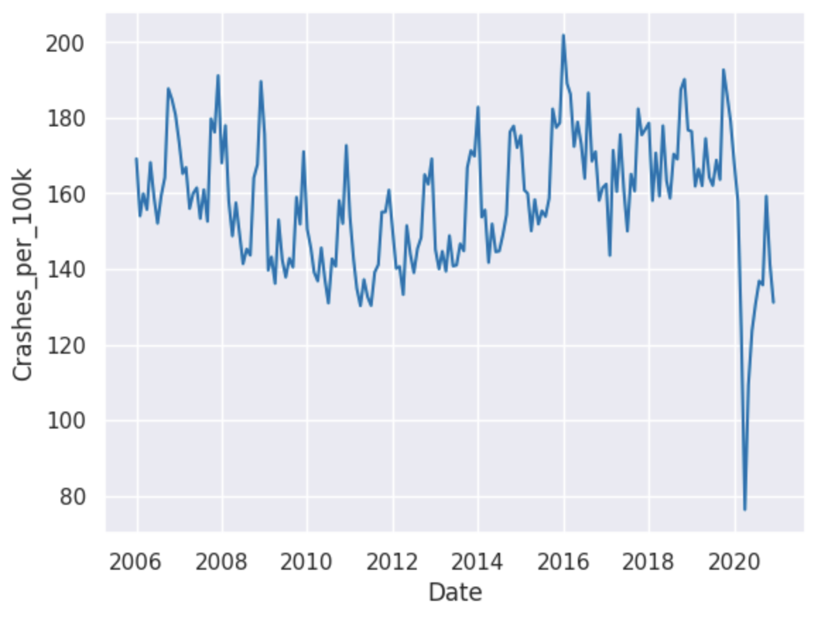
To test this hypothesis, I will calculate the number of crashes per 100,000 people for each year and create a line graph to visualise the trend over time.


    sns.lineplot(x='Date', y='Crashes_per_100k', data=traffic)
    plt.show()

Results

From the line graph, it is clear that there is a general downward trend in the number of crashes per 100,000 people from 2006 to 2012, with crashes increasing again from 2012 to 2020. Looking at the data in 2020, there is a clear outlier where the number of crashes per 100,000 people is significantly lower than in previous years. This could be due to the COVID-19 pandemic, which led to reduced travel and changes in driving behavior. On top of this, each year seems to fluxuate which could be due to seasons throughout the year.

Comparing the data to my hypothesis, my hypothesis is correct after the year 2012. If I wanted to look into this further I would have to look at car production rates over these years and plot a scattergraph with this dataset.

As I noticed there are fluctuations throughout each year, I look further into the crashes per season.

Seasonal Traffic Safety Analysis

Hypothesis

My hypothesis is that the number of crashes will be higher in the winter months due to adverse weather conditions.

Method

To test this hypothesis, I will calculate the number of crashes per 100,000 people for each season and create a boxplot to visualise the trend.


    sns.boxplot(x='Crashes_per_100k', y='Season', data=traffic[traffic.Date.dt.year!=2020])
    plt.show()

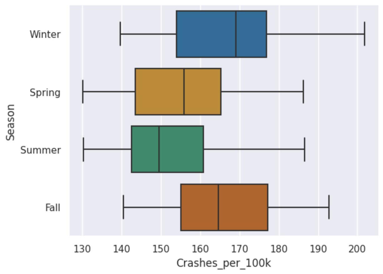
Results

From analysing the boxplot, winter has the highest number of crashes at over 200 crashes per 100,000. Additionally, the median number of crashes in winter is higher than in the other seasons at almost 170 per 100,000, indicating that winter tends to have more crashes overall and thus helping to prove my hypothesis.

Looking at the other seasons, autumn has the second highest median number of crashes, followed by spring and then summer. This could be due to a variety of factors, such as weather conditions, road conditions, and driver behavior during different seasons.

Futhermore, you can clearly see that the interquartile range (IQR) for winter is similarly sized to autumn's IQR and spring's IQR but the IQR for summer is smaller. This suggests that while winter has the highest number of crashes, the variability in crash numbers is similar to that of autumn and spring, whereas summer has less variability in crash numbers.

Overall, this boxplot provides valuable insights into the seasonal patterns of traffic crashes and can help inform strategies for improving road safety during different times of the year.

Smartphone and Traffic Safety Data Inspection

To invetigate the correlation between smartphone ownership and traffic accidents, I have a dataset that has both tables in.


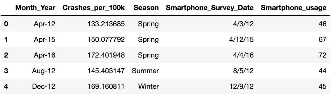
    smartphones=pd.read_csv('crashes_smartphones.csv')
    smartphones.head()

Check the datatypes of the columns to ensure they are correctly formatted.


    smartphones.info()

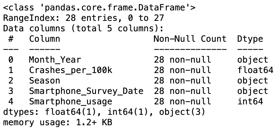
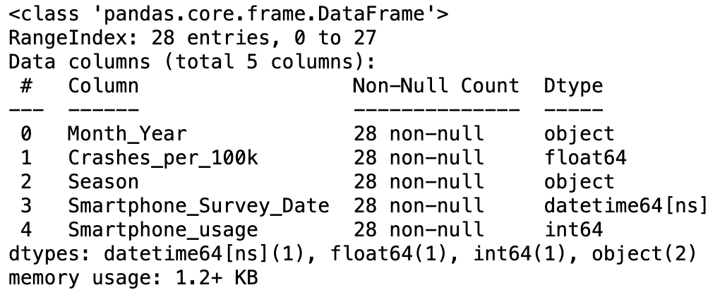
Change the datatype of the 'Year' column to datetime format.


    smartphones['Smartphone_Survey_Date']=pd.to_datetime(smartphones['Smartphone_Survey_Date'])
    smartphones.dtypes

Looking at the data for smartphones and traffic safety, traffic safety has 180 rows compared to only 28 in smartphones, luckily neither dataset has missing data. Sample size can affect results and make the conclusions drawn from them less reliable.

Visualising Smartphone Data

Hypothesis

My hypothesis is that over time smartphone usage will increase due to technological developments and phones becoming more of an essential item than a luxury.

Method

To test this hypothesis, I will create a line graph to visualise the trend of smartphone usage over time.


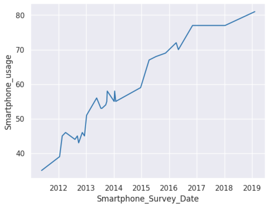
    sns.lineplot(x='Smartphone_Survey_Date', y='Smartphone_usage', data=smartphones)
    plt.show()

Results

From the line graph, it is clear that there is an upward trend in smartphone usage from 2011 to 2019, with smartphone usage increasing from around 30 in 2011 to around 80 in 2019. This supports my hypothesis that smartphone usage will increase over time due to technological developments and phones becoming more of an essential item than a luxury.

Correlation Between Smartphone Usage and Traffic Accidents

Hypothesis

My hypothesis is that as smartphone usage increases, the number of traffic accidents will also increase due to distracted driving.

Method

To test this hypothesis, I will plot smartphone usage against the number of crashes per 100,000 people on a scattergraph. I will also plot a line of best fit in order to visualise the correlation between the two variables.


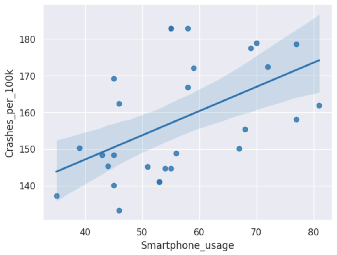
    sns.regplot(x='Smartphone_usage', y='Crashes_per_100k', data=smartphones)
    plt.show()

I will also calculate the Pearson's correlation coefficient and the associated p-value.


    corr, p = pearsonr(smartphones.Smartphone_usage, smartphones.Crashes_per_100k)
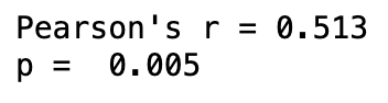
    print("Pearson's r =",  round(corr,3))
    print("p = ", round(p,3))

Results

From the scattergraph, we can visually see there is a positive correlation between smartphone usage and the number of crashes per 100,000 people, with a Pearson's r value of 0.513. This indicates a moderately strong positive correlation between the two variables, suggesting that as smartphone usage increases, the number of traffic accidents also tends to increase.

The p-value of 0.005 indicates that this correlation is statistically significant, meaning that it is unlikely to have occurred by chance. Therefore, I can reject the null hypothesis and conclude that there is a significant correlation between smartphone usage and the number of traffic accidents.

Overall, these results support my hypothesis that as smartphone usage increases, the number of traffic accidents will also increase due to distracted driving.

Linear Regression Analysis

Outlier Prediction

As noted previously, there is a clear outlier in number of crashes per 100,000 in the year 2020, which is significantly lower than in previous years. This could be due to the COVID-19 pandemic, which led to reduced travel and changes in driving behavior. Therefore, I will exclude this data point from the linear regression analysis in order to avoid skewing the results. Then I shall compare the results of the linear regression analysis with and without the outlier to see how it affects the results.

Method

First I shall prepare the data for linear regression and look at the y-intercept and the gradient of the linear regression line equation.


    X = smartphones['Smartphone_usage'].to_numpy().reshape(-1, 1)
    y = smartphones['Crashes_per_100k'].to_numpy().reshape(-1, 1)

    lm=LinearRegression()
    lm.fit(X, y)

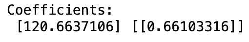
    print("Coefficients: \n",lm.intercept_, lm.coef_)

Using the y-intercept and gradient, I can make a prediction of where 2020 would be if it followed the same pattern.


    y_pred=lm.intercept_ + lm.coef_*80
    print("My 2020 crash prediction is", y_pred)

Next I will plot both the predicted value and the actual value on the previous regression plot to see how differing the results are.


    sns.regplot(x = 'Smartphone_usage', y = 'Crashes_per_100k', data = smartphones)
    sns.scatterplot(x=[81,81], y=[174.20,157.89], hue=['predicted','actual'], 
        style=['predicted','actual'], markers=['X','o'], palette=['navy','orange'], s=200)
    plt.legend(title='2020')
    plt.show()

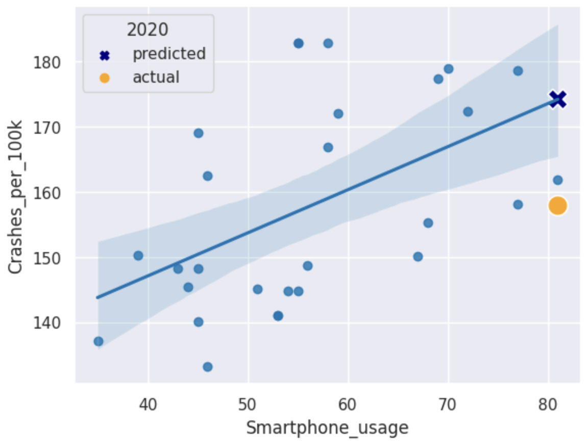
Results

From the coefficients of the linear regression line, we can see that the y-intercept is 120.664 (3dp) and the gradient is 0.661 (3dp).

Using these coefficients, I predicted that if smartphone usage was 80% in 2020, the number of crashes per 100,000 people would be approximately 174 (nearest integer). However, the actual number of crashes per 100,000 people in 2020 was only 157.89, which is significantly lower than the predicted value. This suggests that there were other factors at play in 2020 that led to a decrease in traffic accidents, such as reduced travel and changes in driving behavior due to the COVID-19 pandemic.

Overall, this analysis highlights the importance of considering external factors when interpreting data and making predictions.

Conclusion

Project Oveview

The central aim of this project was to test the hypothesis that as smartphone usage increase, the number of traffic accidents will also increase due to the effects of distracted driving. Through a detailed analysis involving time-series data, correlation studies, and regression modeling, the findings robustly confirm a statistically significant positive correlation, thereby supporting the hypothesis. However, the comprehensive investigation also highlighted the critical role of external, confounding variables that modify this relationship in real-world scenarios, demanding a nuanced interpretation of the initial findings.

Validation of the Core Hypothesis

The primary statistical evidence for the hypothesis stems from the correlation analysis between smartphone usage (measured as percentage of ownership/usage) and the rate of crashes per 100,000 people. The scattergraph analysis yielded a Pearson's r value of 0.513. This metric signifies a moderately strong positive correlation between the two variables. Statistically, this means that as the measured prevalence of smartphone use rises, there is a distinct tendency for the frequency of traffic accidents to rise alongside it. This quantitative relationship directly backs the underlying premise of the hypothesis—that the increasing availability of handheld devices leads to a corresponding increase in the distraction-related risks associated with driving.

Crucially, the statistical significance of this correlation was established by the derived p-value of 0.005. Because this p-value is far less than the conventional significance level of 0.05, we can confidently reject the null hypothesis, which would have proposed no relationship exists. The low p-value confirms that the observed positive relationship is highly unlikely to have occurred by chance, thus establishing a legitimate statistical link. The overall conclusion drawn from this core statistical analysis is definitive: a significant positive correlation exists between smartphone usage and the number of traffic accidents, directly supporting the project's foundational hypothesis, especially for the time period following 2012 where the accident trend aligns more closely with the consistent upward trend in device usage.

Interpreting the Linear Regression Model

The exploration extended beyond simple correlation into predictive modeling using a linear regression line, the coefficients of which offer deeper insight into the quantitative relationship. The calculated linear regression line was defined by a y-intercept of 120.664 (to 3 decimal places) and a gradient of 0.661 (to 3 decimal places).

Using the derived model, a projected smartphone usage of 80% in 2020 led to a predicted accident rate of approximately 174 crashes per 100,000 people. However, the actual recorded rate for 2020 was significantly lower at 158. This substantial divergence between prediction and reality provides a powerful demonstration that correlation does not equate to sole causation. The model, based on historical trends where the primary explanatory variable was increasing smartphone usage, failed to account for a dramatic, unprecedented external shock to the system: the COVID-19 pandemic.

The Influence of Contextual Factors: Pandemic and Seasonal Effects

The discrepancy observed in 2020 necessitates the discussion of confounding variables. The reduced traffic accidents in 2020, despite high smartphone usage, is attributed to external factors such as reduced travel, widespread lockdowns, and fundamental changes in driving behaviour. With fewer vehicles on the road, the statistical probability of accidents decreases, regardless of individual driver distraction levels. This highlights a crucial caveat in the hypothesis: while distracted driving may increase the risk per driver-mile, a global reduction in total driver-miles can override this effect on the macro-level accident count. This finding underscores the necessity of incorporating macroeconomic and societal variables when creating robust predictive models for traffic safety.

In addition to the pandemic’s influence, the project’s exploration into crash rates over time and across seasons further enriched the contextual understanding. The time-series data for crashes from 2006 to 2020 initially showed a general downward trend from 2006 to 2012, followed by an increasing trend up to 2019 (before the 2020 outlier). This non-linear pattern suggests that multiple factors are at play, including car production rates, vehicle safety technology improvements, and changing infrastructure, which competed with the distraction effect in the earlier part of the observed decade.

The seasonal analysis provided yet another layer of complexity. The boxplot visualization clearly indicated that winter has the highest median number of crashes (approximately 170 per 100,000 people), followed by autumn, spring, and finally summer. This strongly suggests that factors like adverse weather conditions (ice, snow, rain, reduced visibility) are potent accident multipliers, surpassing even the consistent factor of human-induced smartphone distraction in terms of median accident rate. The seasonal variability illustrates that the hypothesis, while statistically verified, operates within a dynamic system where environmental and road conditions significantly modulate the final outcome.

Reflection and Future Research Directions

In summary, the project successfully validated the hypothesis through strong statistical evidence: increased smartphone usage is significantly and positively correlated with a rise in traffic accidents. This supports the general public health concern regarding distracted driving.

However, the analysis also demonstrated that the relationship is not one of simple, isolated causation. The predictive model was vulnerable to external shocks (the pandemic) and its real-world expression is heavily influenced by systemic factors (seasonal weather).

For future research, several avenues could be explored to build upon these findings:

Refined Variable Measurement: Instead of relying on overall smartphone usage, future studies should seek data that more directly measures distracted driving behaviour (e.g., tickets issued for phone use, or real-time data from driving apps).
Multivariate Modeling: To create a truly robust predictive model, the linear regression should be expanded into a multiple regression model to incorporate confounding variables identified here, such as seasonal indicators, vehicle miles traveled (VMT), and economic indicators (e.g., employment rates affecting commuting).
Longitudinal Study of Legislation: An interesting follow-up would be to study the impact of specific anti-distracted driving laws introduced in various jurisdictions, analyzing the change in the correlation coefficient before and after the legislation’s implementation.

Ultimately, while the statistical link is undeniable, the conclusion of this project is that tackling distracted driving requires a holistic approach that integrates technology, policy, driver education, and an acknowledgement of the environmental and societal contexts in which driving occurs.